Performance

The headline claim — millisecond-scale aggregation in the hot path — is backed by a reproducible suite in benchmarks/. This page reads the numbers; the full generated report has every row.

uv run python -m benchmarks.run

The shape of the cost

geohalo deliberately moves all the expensive work into a one-time precompute, leaving a hot path that applies a precomputed sparse matrix to the grid values.

flowchart LR
    subgraph once ["once — seconds"]
        S["Stencil / ReduceOperator build<br/>exactextract + sparse assembly"]
    end
    subgraph each ["per grid slice — milliseconds"]
        M["sparse products<br/>bounded batches or individual slices"]
    end
    S -.cache.-> M

Precompute — pay once

Building the stencil scales with polygon count and vertex complexity; the resulting matrix is small and cacheable.

n_polygons (GADM Brazil L2)	Stencil.compute	CSR size
50	~21 ms	6 KB
507	~170 ms	38 KB
5571	~2.1 s	430 KB

After the first build, a cache hit loads in milliseconds — a ~30–46× speedup for stencils, and thousands of times for a refined ReduceOperator.

Detailed polygons: WKB versus GeoJSON

The synthetic benchmark for #7 isolates stencil construction with detailed boundaries:

uv run python -m benchmarks.stencil_build

On 3,000 synthetic polygons with 6,003,000 vertices and a global 0.25° grid, a local run measured these medians over three complete builds:

Geometry input	Build time
Previous GeoJSON path	15.731 s
Current WKB path	1.079 s

This was a 14.6× speedup, with identical CSR matrices, row sums, polygon keys, and cache digests. Both paths include sorting, geometry serialization, exactextract coverage, sparse assembly, and hashing; polygon generation is excluded. The WKB path also reuses its encoded geometries for the digest.

Environment: Python 3.14.4, exactextract 0.3.0, Shapely 2.1.2, NumPy 2.4.6, SciPy 1.17.1, and GeoPandas 1.1.3. Timings depend on hardware and polygon complexity; the earlier GADM table uses different polygons and is a separate historical measurement.

Hot path — pay per slice

All rows below aggregate to GADM Brazil L2 (~5570 municipalities) on a 0.25° grid over Brazil (160×160 = 25 600 cells). The batch dims are arbitrary — any stacked non-spatial dims work; here they follow the ECMWF data the suite happens to use, where member=50 is a 50-member ensemble and step=N is N lead times.

n_polygons	batch	slices	factor	median
50	(member=50,)	50	1	3.6 ms
5571	(member=50,)	50	1	5.8 ms
5571	(member=50, step=10)	500	1	196 ms
5571	(member=50, step=40)	2 000	1	670 ms
5571	(member=50,)	50	4 (refined)	113 ms
5571	(member=50,)	50	1 (1 % NaN)	14 ms

A batch of 50 grid slices over 5 571 polygons reduces in single-digit milliseconds. The cost scales with the number of slices, and the NaN-aware path costs roughly 2–3× the clean path for its second matmul.

Large-grid application memory

The synthetic benchmark for #5 runs without external data:

uv run python -m benchmarks.operator_memory

It compares the previous sort-and-batch implementation with the current application path on a global 0.25° grid: 24 float32 slices (95.05 MiB), 90 polygons, and 15,210 matrix coefficients. A local run produced:

Latitude order	Previous extra peak	Current first-call peak	Current warm peak	Previous median	Current median
Ascending	285.2 MiB	0.540 MiB	0.263 MiB	78.00 ms	3.16 ms
Descending	475.3 MiB	0.545 MiB	0.326 MiB	134.26 ms	2.56 ms

Results were identical in this run, retaining float64 arithmetic. Peaks are tracemalloc allocations during application, including output and any first-call preparation, but excluding the already allocated input and canonical matrix. They are not total process RSS. Timings are warmed medians of five calls and vary by hardware. The benchmark checks results against the previous product at rtol=1e-12 and atol=1e-12.

The fusion win

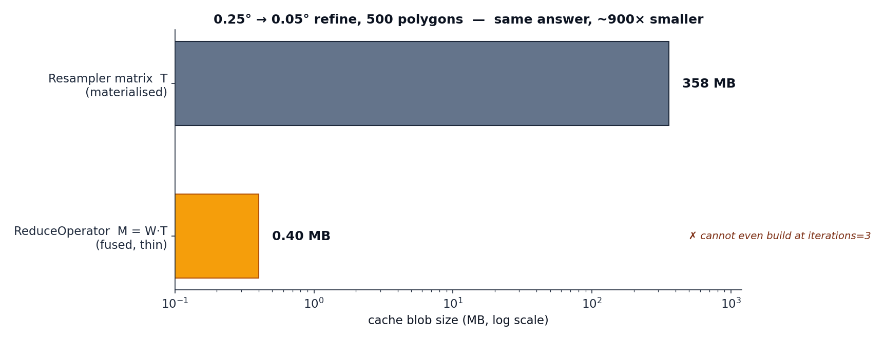
For a 0.25° → 0.05° refine (~3.2 M target cells) over 500 polygons, the materialised resampler is a 358 MB blob that cannot build at all at iterations=3. The fused ReduceOperator is a 0.40 MB blob, builds in ~0.5 s, and loads in ~0.5 ms — same answer, ~900× smaller.

Chunk-aware reads

RestrictedOperator addresses the remaining full-grid I/O cost for clean lazy inputs. The synthetic #6 benchmark uses a local in-memory Zarr v3 store and counts actual data-chunk reads:

uv run python -m benchmarks.chunk_reads

For 24 float32 steps on a descending 721 × 1440 grid, 15 polygons in two distant regions, and storage chunks of 6 × 64 × 64, a local run measured:

Path	Data-chunk reads	Compressed payload read	Extra allocation peak	Median time
Full-grid reduce_with_operator	1,104	84.747 MiB	98.388 MiB	1.0690 s
reduce_with_restricted_operator	12	1.003 MiB	0.467 MiB	0.0277 s

The plan reads two disjoint windows covering 12,288 of 1,038,240 spatial cells (1.18%). Every fetched data chunk was read once, and outputs matched exactly in this run. The benchmark asserts agreement at rtol=1e-12, atol=1e-12.

Times are medians of three uninstrumented applications; the extra peak is from a separate tracemalloc run, not total process RSS. Data generation, store creation, coordinate loading, and operator construction are excluded. This is local decoding and reduction, not a cloud latency measurement. Physical I/O also depends on storage chunking, sharding, and any upstream Dask transformations.

Environment: Python 3.14.4, xarray 2026.4.0, Zarr 3.4.0, NumPy 2.4.6, SciPy 1.17.1, Intel Core Ultra 5 125H in a Linux virtual machine. The application uses Zarr without Dask here; tests also count actual reads through Dask-backed Zarr and irregular Dask chunks.

Rollups

Hierarchical rollups are another matmul. The full GADM Brazil muni → state hierarchy (5 571 leaves) rolls a batch of 50 slices up in ~5.6 ms; with a 500-slice batch, ~19 ms.

Tree construction

The synthetic benchmark for #8 compares the previous row-by-row builder with the depth-bounded sparse builder:

uv run python -m benchmarks.bias_tree_build
uv run python -m benchmarks.bias_tree_build --leaves 5570 --fanout 10
uv run python -m benchmarks.bias_tree_build --leaves 20000 --fanout 10 --repeats 1

Local measurements of complete builds, including validation, ordering, matrix assembly, and hashing (but excluding synthetic hierarchy generation). The first two tree sizes use medians of three builds; the largest uses one build per mode:

Leaves	Internal nodes	Mode	Previous build	Sparse build
2,862	25	weighted mean	1.015 s	0.022 s
2,862	25	weighted sum	1.092 s	0.013 s
5,573	620	weighted mean	2.905 s	0.055 s
5,573	620	weighted sum	3.201 s	0.034 s
20,003	2,223	weighted mean	30.307 s	0.194 s
20,003	2,223	weighted sum	29.787 s	0.142 s

The benchmark checks exact equality of CSR coefficients, indices, row pointers, node keys, and cache digests for both modes. Each hierarchy includes three leaves attached directly to the root, exercising unequal leaf depths. Build cost depends on depth and the number of contributing leaf–ancestor pairs, not just leaf count.

Environment: Python 3.14.4, NumPy 2.4.6, pandas 3.0.3, SciPy 1.17.1, Intel Core Ultra 5 125H in a Linux virtual machine. Timings vary with machine load; these are synthetic build measurements, separate from the historical GADM hot-path timings.

Caveats

Numbers are point-in-time on the author's machine and vary ±20 % by hardware. Cold-import overhead (~0.3 s for import geohalo) is excluded — the suite measures steady-state cost. The full report is regenerated after any perf-relevant change and records the exact environment, hardware, and methodology.