The fused reduce operator

When you reduce over a refined grid, two linear maps stand between the source data and the answer: a resampler \(\mathbf{T}\) (source → fine grid) and a stencil \(\mathbf{W}\) (fine grid → polygons).

\[ \mathbf{a} \;=\; \mathbf{W}\,(\mathbf{T}\,\mathbf{x}) \;=\; (\mathbf{W}\mathbf{T})\,\mathbf{x} \]

The naive route builds \(\mathbf{T}\), applies it to make a fine field, then applies \(\mathbf{W}\). But \(\mathbf{T}\) spans the entire fine grid — millions of cells — even though only the handful of cells under each polygon will ever survive the multiplication by \(\mathbf{W}\). That is enormous wasted work and memory.

The fusion

By associativity, the two operators compose into one:

\[ \mathbf{M} \;=\; \mathbf{W}\mathbf{T} \;\in\; \mathbb{R}^{N_\text{polygons} \times N_\text{source}} \]

\(\mathbf{M}\) acts directly on the source grid. It has only \(N_\text{polygons}\) rows, so it is tiny — and crucially, geohalo builds it without ever materialising \(\mathbf{T}\). FactoredResampler.fuse_left(W) pushes the thin \(\mathbf{W}\) through the resampler's factored form:

\[ \mathbf{T} = \mathbf{y}_\text{op} + \mathbf{P}(\mathbf{I} - \mathbf{A}\mathbf{y}_\text{op}), \quad \mathbf{y}_\text{op} = \Bigl(\textstyle\sum_j \mathbf{G}^j\Bigr)\mathbf{B} \]

\[ \Longrightarrow\quad \mathbf{W}\mathbf{T} = \mathbf{W}\mathbf{P} + (\mathbf{W} - \mathbf{W}\mathbf{P}\mathbf{A})\Bigl(\textstyle\sum_j \mathbf{G}^j\Bigr)\mathbf{B} \]

and the series is accumulated by right-applying \(\mathbf{G}\) to the thin \((\mathbf{W} - \mathbf{W}\mathbf{P}\mathbf{A})\). Every intermediate keeps only \(N_\text{polygons}\) rows, so the fusion scales to high iteration counts and huge target grids where \(\mathbf{T}\) itself would not fit in memory.

flowchart LR
    subgraph naive ["naive: build the fine grid"]
        direction LR
        X1["source x"] -->|"T (N_target × N_source)"| FINE["fine field<br/>millions of cells"]
        FINE -->|"W"| A1["a"]
    end
    subgraph fused ["fused: one thin operator"]
        direction LR
        X2["source x"] -->|"M = W·T<br/>(N_poly × N_source)"| A2["a"]
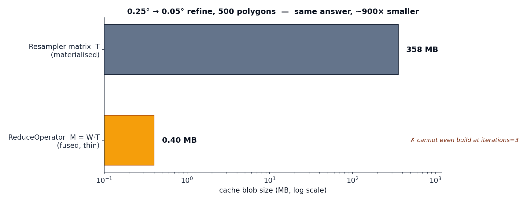
    end

Why it matters: the size win

The fused operator is the most compact thing to cache, and — unlike \(\mathbf{T}\) — its size does not grow with target resolution or iteration count.

A 0.25° → 0.05° refine (~3.2 M target cells) over 500 polygons. The materialised resampler is a 358 MB cache blob that cannot even build at iterations=3. The fused ReduceOperator is 0.40 MB, builds in ~0.5 s, and loads in ~0.5 ms — the same answer, roughly 900× smaller.

ReduceOperator

ReduceOperator.compute(stencil, source_lat, source_lon, iterations=…) returns the stencil's own matrix unchanged when the source grid already matches the stencil grid (no resample needed), and otherwise calls fuse_left. Applying it is a single matmul on the source grid:

import geohalo as ghl

op = cache.get_or_compute_reduce_operator(
    stencil, da.latitude.values, da.longitude.values, iterations=3,
)
out = ghl.reduce_with_operator(da, op)     # (..., geom); also accepts how="sum"

Clean data only

reduce_with_operator assumes non-NaN, unweighted data — the fused operator bakes in a fixed normaliser and cannot renormalise per cell. For missing values or per-cell weights, use reduce_with_stencil, which keeps the resampler factored and renormalises each slice.

It's already your fast path

You rarely call this directly. reduce and reduce_with_stencil use exactly this fusion internally for clean data: they build a ReduceOperator once and delegate to reduce_with_operator. The reason to cache the operator yourself is repetition — if you apply the same (stencil, source grid, iterations) across many grid slices (time steps, members, bands) or repeated runs, caching the fused operator skips even the (cheap) fusion step and loads a sub-millisecond blob. See caching.