Mean-preserving downscaling

Many polygons are smaller than a single grid cell. Exact coverage will still answer — it returns the value of the cell the polygon sits in — but that answer is flat across the whole cell. geohalo can do better by refining the grid first, using neighbouring cells to give sub-cell polygons a sharper estimate.

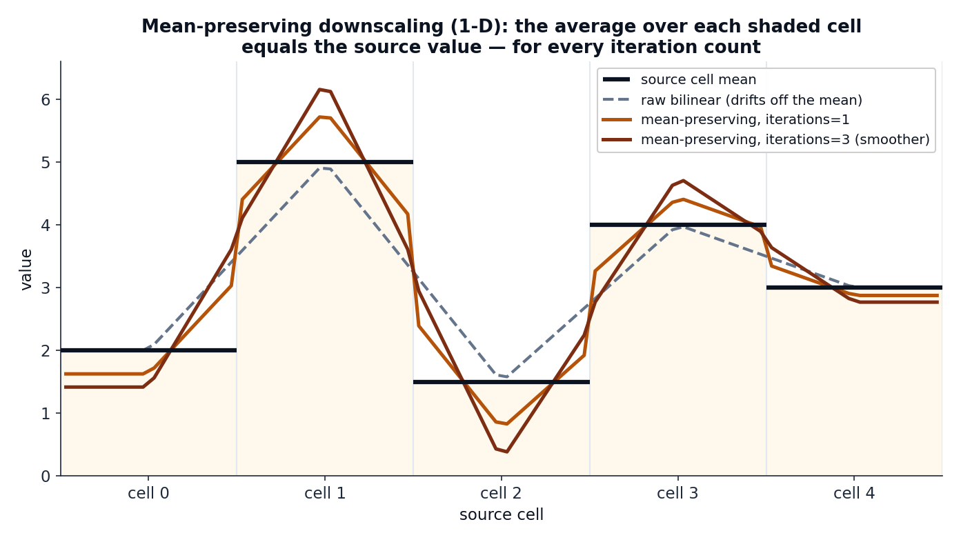
The catch: a naive upsample (plain bilinear) drifts off the published cell mean. geohalo's Resampler refines without breaking the contract that the grid encodes — the average of a parent cell's children equals the parent's original value, exactly.

The contract

A gridded field publishes cell means. A refinement that respects this must satisfy, for every source cell \(s\) and its set of target children \(\{t : \pi(t) = s\}\):

\[ \frac{1}{n_s}\sum_{\pi(t)=s} y_t \;=\; x_s \]

Plain bilinear interpolation does not — it smooths across cell boundaries and quietly shifts each cell's average. The figure below shows the gap in one dimension:

A 5-cell source field refined ~16×. Raw bilinear (dashed) is smooth but its average over each cell no longer equals the source value. The mean-preserving curves (amber/rust) add a correction so the integral over every shaded cell returns to the source mean — for any iteration count. More iterations trade a little overshoot for more smoothness.

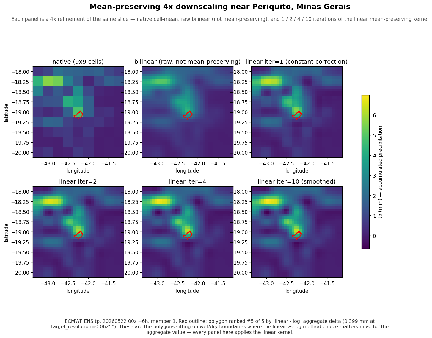
And on a real ECMWF precipitation field over eastern Brazil:

Native cell-mean field, raw bilinear (not mean-preserving), and 1 / 2 / 4 / 10 iterations of the mean-preserving kernel. Every refined panel preserves each parent cell's mean exactly; iterations only change smoothness.

Construction

From the source and target coordinate arrays, geohalo builds three value-independent sparse matrices (geohalo.resampler._build_factors):

• \(\mathbf{B}\) — bilinear interpolation, target ← source. Separable as \(\mathbf{B} = \mathbf{B}_\text{lat} \otimes \mathbf{B}_\text{lon}\), each 1-D factor mapping source centres to target centres with clamped edges (bilinear_matrix_1d).
• \(\pi\) — a nearest-cell assignment of each target cell to its parent source cell (nearest_index). From it:
  • \(\mathbf{P}\) — source → target broadcast: \(P_{t,\pi(t)} = 1\).
  • \(\mathbf{A}\) — source ← target mean: \(A_{s,t} = 1/n_s\) when \(\pi(t) = s\), where \(n_s\) is the number of target cells assigned to source cell \(s\). A source cell with no children has an all-zero row.

The refinement is an interpolate-and-correct loop, linear in the source values \(\mathbf{x}\):

\[ \begin{aligned} \mathbf{y}_0 &= \mathbf{B}\,\mathbf{x} \\[2pt] \text{smooth} \times (\text{iter}-1): \quad \mathbf{y} &\leftarrow \mathbf{y} + \mathbf{B}\,(\mathbf{x} - \mathbf{A}\,\mathbf{y}) \\[2pt] \text{hard correction}: \quad \mathbf{y} &\leftarrow \mathbf{y} + \mathbf{P}\,(\mathbf{x} - \mathbf{A}\,\mathbf{y}) \end{aligned} \]

Each line measures the residual between the source value and the current average of its children (\(\mathbf{x} - \mathbf{A}\mathbf{y}\)) and adds it back — smoothly through \(\mathbf{B}\) during the iterations, then sharply through \(\mathbf{P}\) at the end.

Collapsing to a matrix

Because every step is linear, the whole loop collapses to a single transform \(\mathbf{T}\) with \(\mathbf{y} = \mathbf{T}\mathbf{x}\):

\[ \mathbf{G} = \mathbf{I} - \mathbf{B}\mathbf{A}, \qquad \mathbf{y}_\text{op} = \Bigl(\sum_{j=0}^{\text{iter}-1} \mathbf{G}^{\,j}\Bigr)\mathbf{B}, \qquad \mathbf{T} = \mathbf{y}_\text{op} + \mathbf{P}\,(\mathbf{I} - \mathbf{A}\,\mathbf{y}_\text{op}) \]

Why the mean is preserved exactly

The hard correction is what guarantees the contract. Since \(\mathbf{A}\mathbf{P} = \operatorname{diag}(n_s > 0)\), applying \(\mathbf{A}\) to \(\mathbf{T}\) gives

\[ \mathbf{A}\mathbf{T} = \mathbf{I} \]

on every source cell that has at least one child — i.e. averaging a source cell's target children recovers the source value exactly, for any iteration count. This always holds when refining; when coarsening, a source cell with no assigned target can't be preserved (geometrically unavoidable, and geohalo leaves those rows zero).

The classic operator is the one-iteration case

With iterations = 1 the series has a single term and the transform reduces to the textbook downscaling operator \(\mathbf{M} = \mathbf{B} + \mathbf{P} - \mathbf{P}\mathbf{A}\mathbf{B}\). Higher iteration counts are the N-term generalisation: the correction reaches further across the grid, smoothing the result while still preserving every mean.

Cost: never materialise \(\mathbf{G}\)

\(\mathbf{G} = \mathbf{I} - \mathbf{B}\mathbf{A}\) is an \(N_\text{target} \times N_\text{target}\) operator that densifies under repeated products — forming its powers directly would be ruinous. geohalo never does. It accumulates the series by applying \(\mathbf{G}\) to \(\mathbf{B}\) on the right, so every intermediate stays \(N_\text{target} \times N_\text{source}\):

acc = term = B
for _ in range(iterations - 1):
    term = term - B @ (A @ term)   # term @ G, but kept thin
    acc = acc + term
y_op = acc

The dense \(N_\text{target}^2\) matrix is never built. The build stays sub-second even for large refinements; cost grows with iterations only because the transform fills in as its reach expands. The default iterations = 1 is the cheapest.

Two forms of the resampler

geohalo ships the transform in two shapes for two different needs:

Class	Holds	compute cost	Use when
Resampler	the materialised \(\mathbf{T}\)	builds the full series	you want the refined grid itself
FactoredResampler	just \(\mathbf{B}, \mathbf{A}, \mathbf{P}\)	only the three base ops	you only want per-polygon values (the reduce path)

Resampler is what resample_grid returns. FactoredResampler is the key to the fused reduce operator: its fuse_left(W) computes \(\mathbf{W}\mathbf{T}\) without ever materialising \(\mathbf{T}\), so refining to a multi-million-cell grid stays cheap.

Using it

import geohalo as ghl

fine = ghl.resample_grid(da, target_resolution=0.05, iterations=3)

Or, through reduce, when the refinement is only a stepping stone to per-polygon values:

out = ghl.reduce(da, geoms, target_resolution=0.05, resample_iterations=3)

In the second form geohalo never builds the fine field at all — it fuses the resample into the stencil. That is the subject of the next page.